Regression is a supervised machine learning method that is used to determine numerical values. This value, is called in ML terms a label. An analogy that can be considered here is a car manufacturing company that would predict the price (label) of a car based on the number of seats, engine size, options, etc. In ML terms, it’s features.
With regression (a supervised ML technique), you would train a model using data that already includes both the features and the labels. With training, the model would learn how to match the features to the labels, therefore, after the model is trained it will be able to predict labels for datasets which only contain features.
Microsoft Azure Machine Learning designer facilitates the creation of such a regression model.
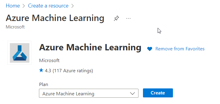
First we need to create the Machine Learning workspace in Azure. Select Create a resource and search for Machine Learning.
Next, fill in the necessary fields.
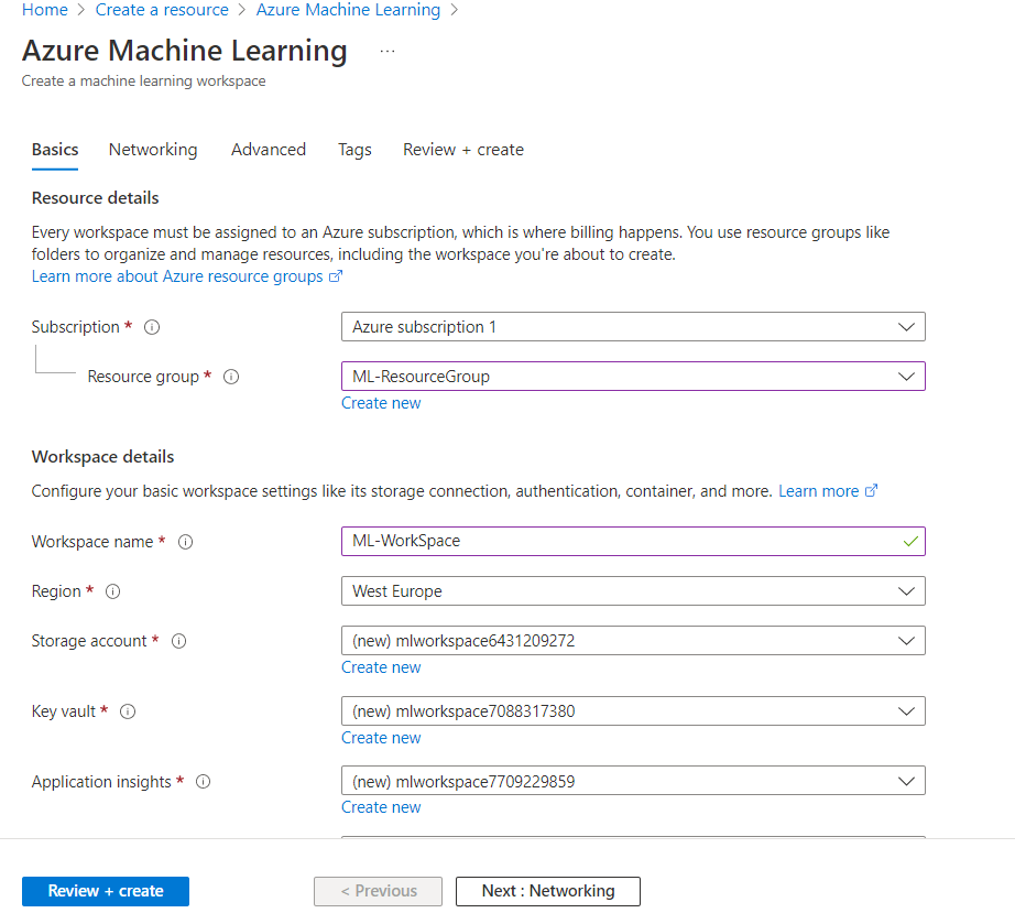
Review, Validate and Create the resource.
Next, open the Azure ML Studio, (or open a new browser tab and navigate to https://ml.azure.com),

In the Compute section on the lower left, we will see four types of compute resources.
- Compute Instances: Development workstations that data scientists can use to work with data and models.
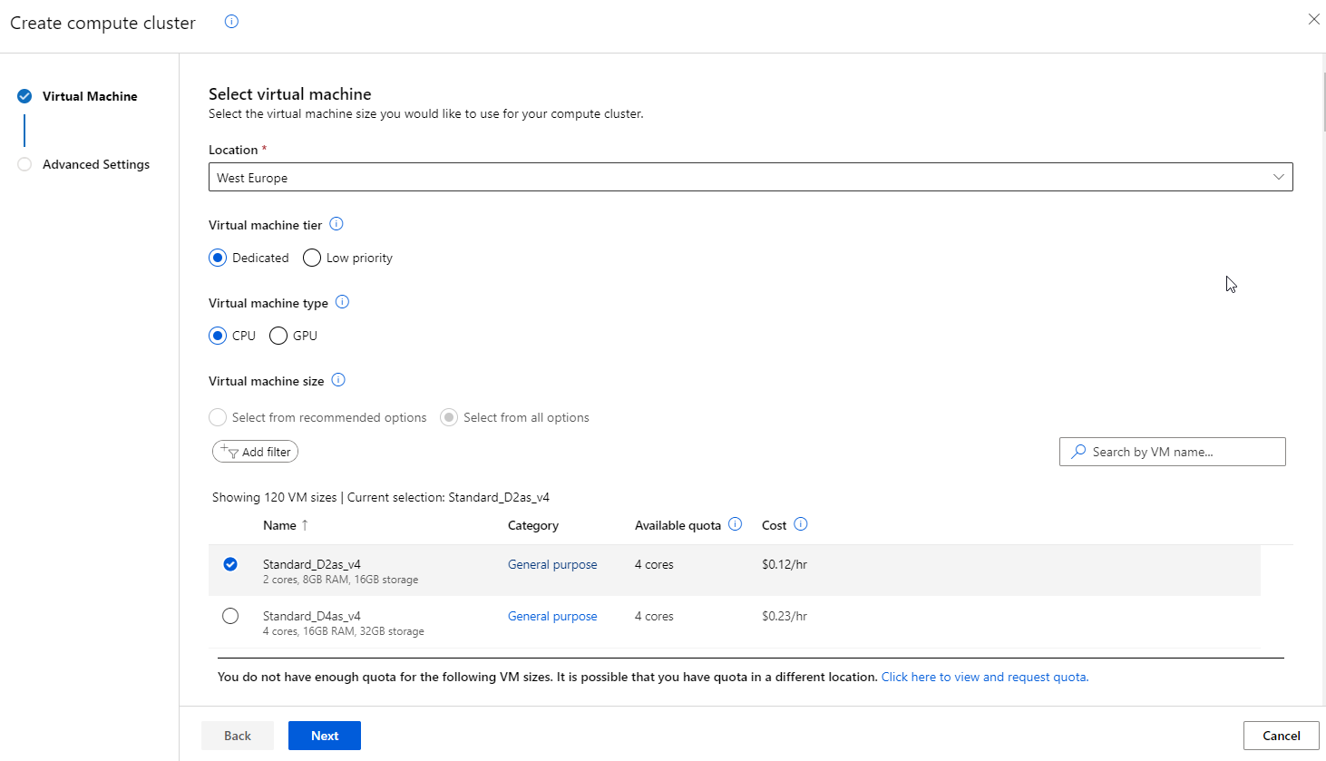
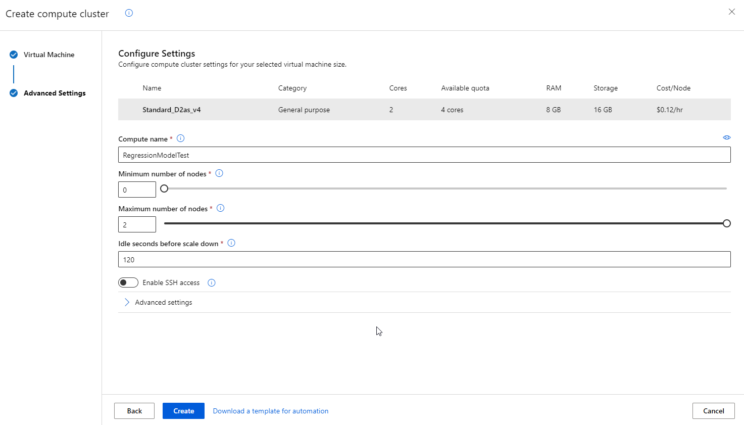
- Compute Clusters: Scalable clusters of virtual machines for on-demand processing of experiment code.
- Inference Clusters: Deployment targets for predictive services that use your trained models.
- Attached Compute: Links to existing Azure compute resources, such as Virtual Machines or Azure Databricks clusters.
In this scenario we will go with the Compute clusters option.
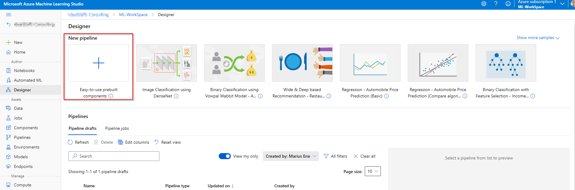
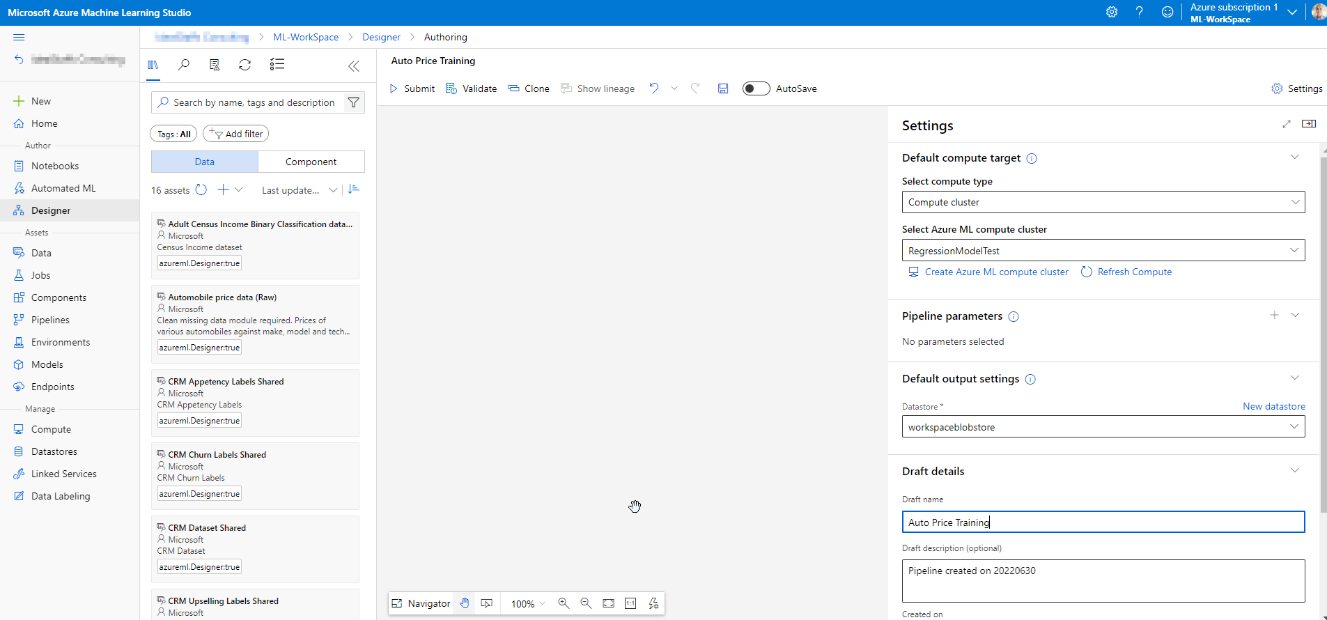
If we want to use the Azure ML Designer feature, its necessary that we create a pipeline for training the machine learning model. Select the new pipeline with blank settings.
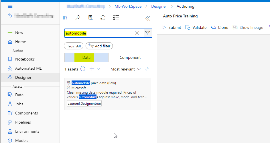
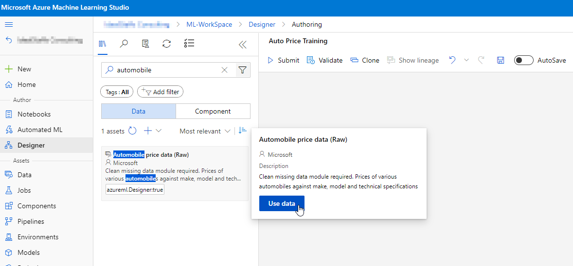
Use the filter to search the Data section for Automobile price data (Raw).
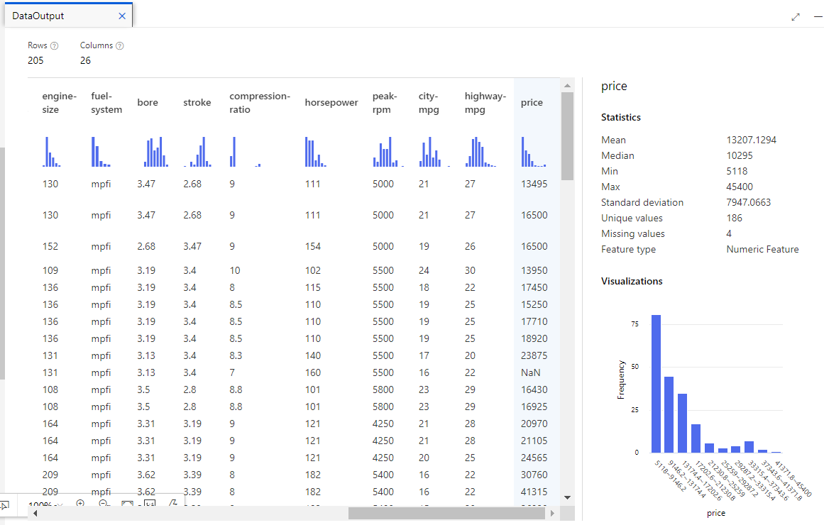
On the canvas, right click and select Preview data.

Review the price information.
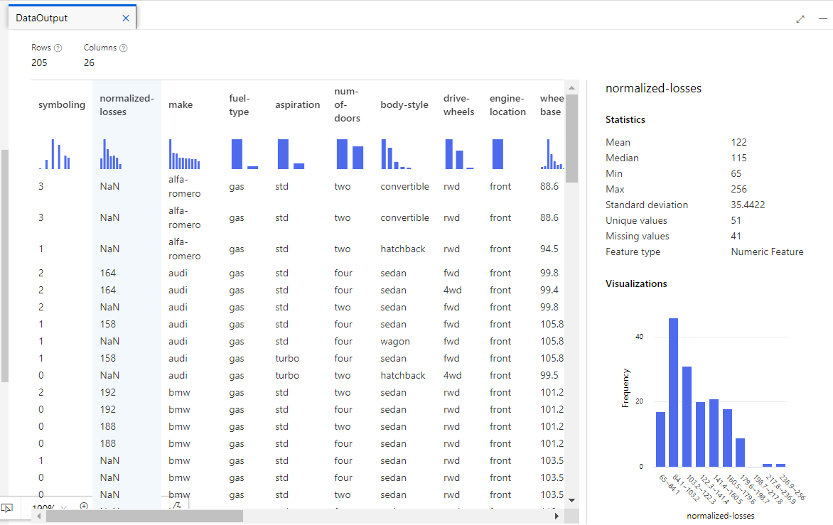
Now revise the normalized losses column. Note that there are a lot of values missing (NaN). This could have a negative impact on the prediction so we might want to exclude it from training.
Now we would apply data transformation to prepare the data for modeling to address the issues identified.
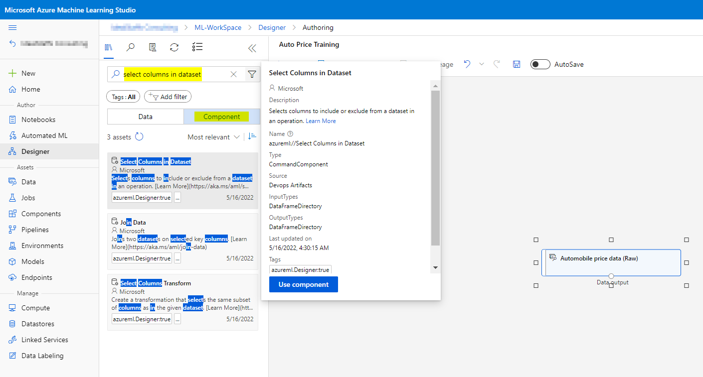
After adding the module to the canvas, connect it with the data component.
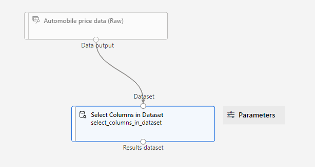
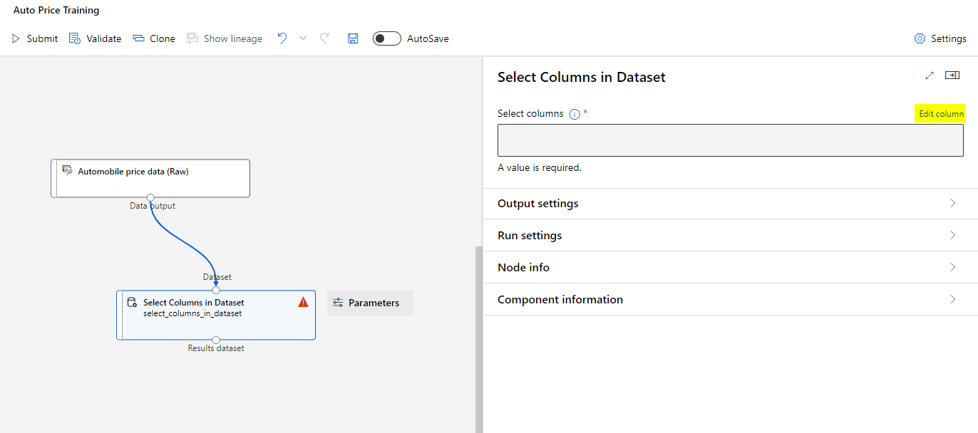
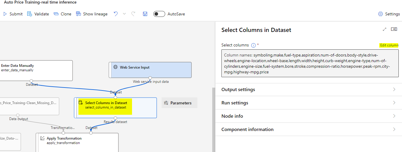
Double click the Select Columns in Dataset module and click Edit column.
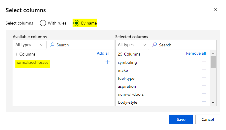
Select By Name and add all columns. You can now exclude the normalized-losses column.
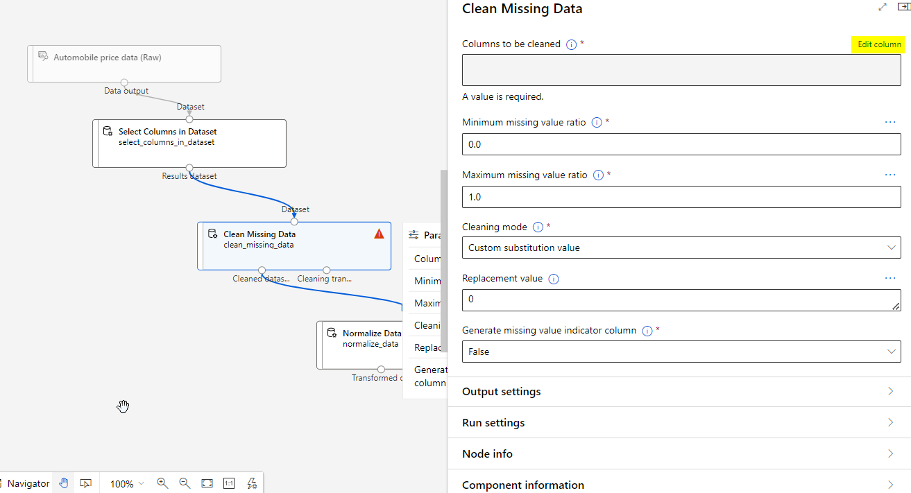
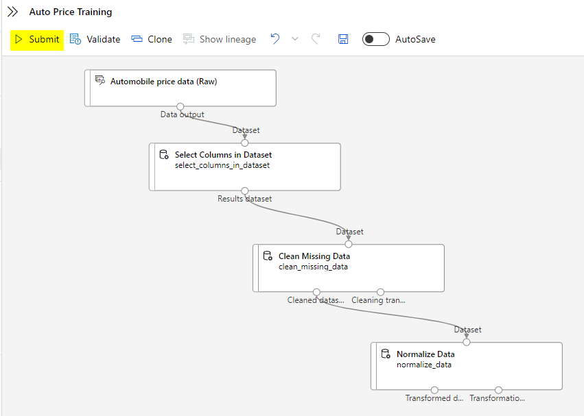
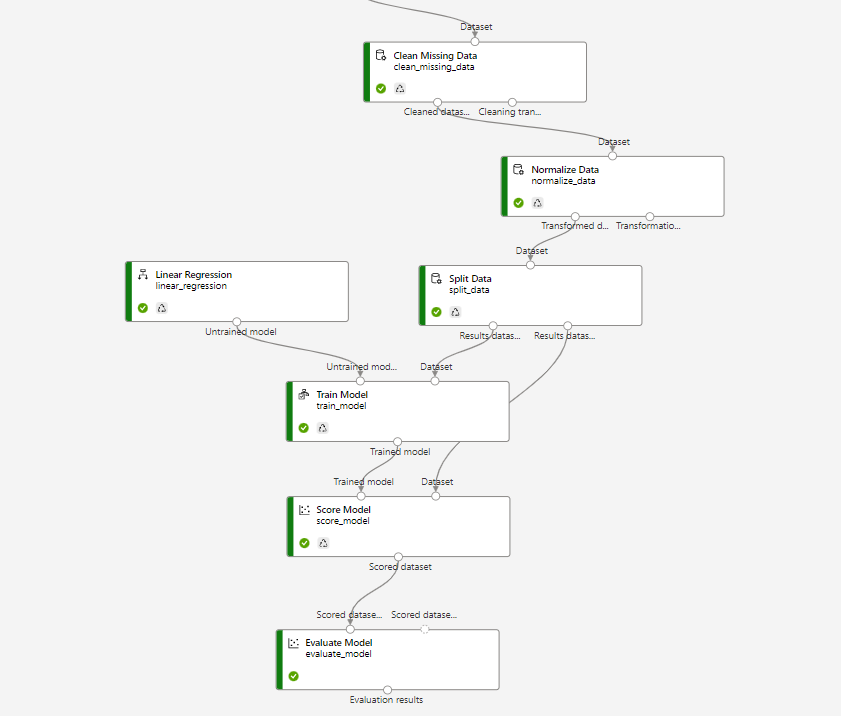
Continue building the pipeline as depicted below:

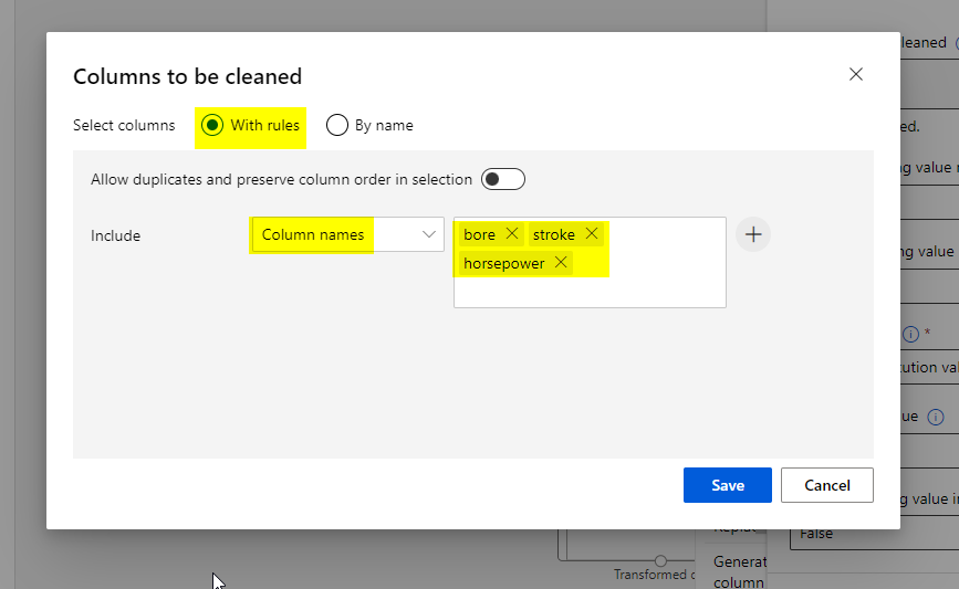
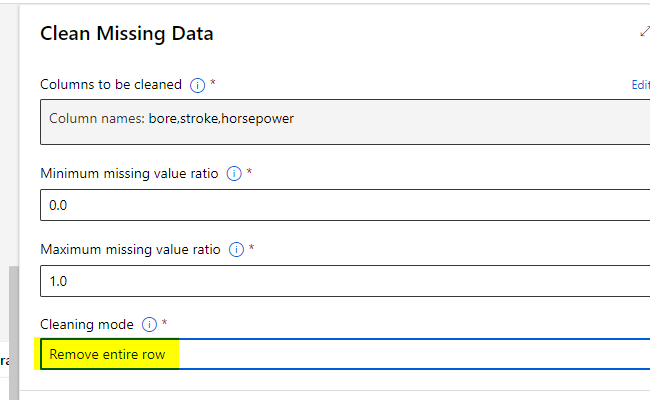
Double click the Clean Missing Data module and click the Edit column.
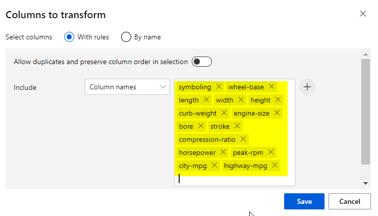
Finally, double click the Normalize Data module and Edit the column and use the MinMax transformation method.
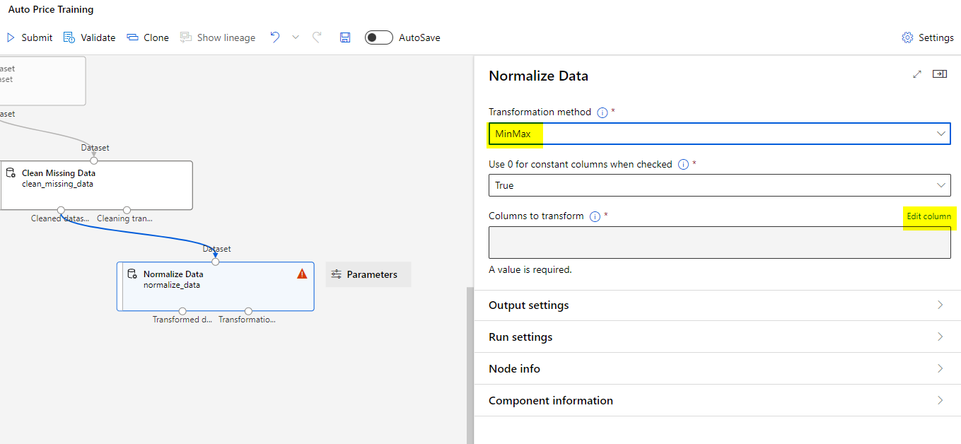
Select the columns from the image to include in the transformation.
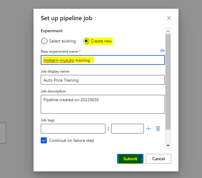
Submit the job to the pipeline.
Wait for the run to finish, which might take 5 minutes or more.
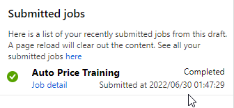
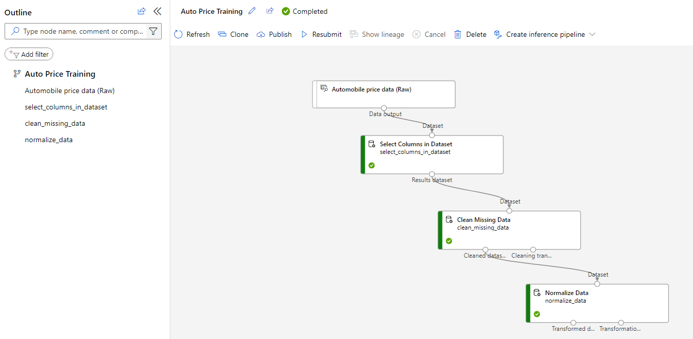
The dataset is now prepared for model training. Close the Job detail window to return to the pipeline.
After using data transformations to prepare the data, its time to train a machine learning model.
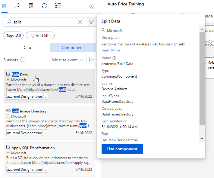
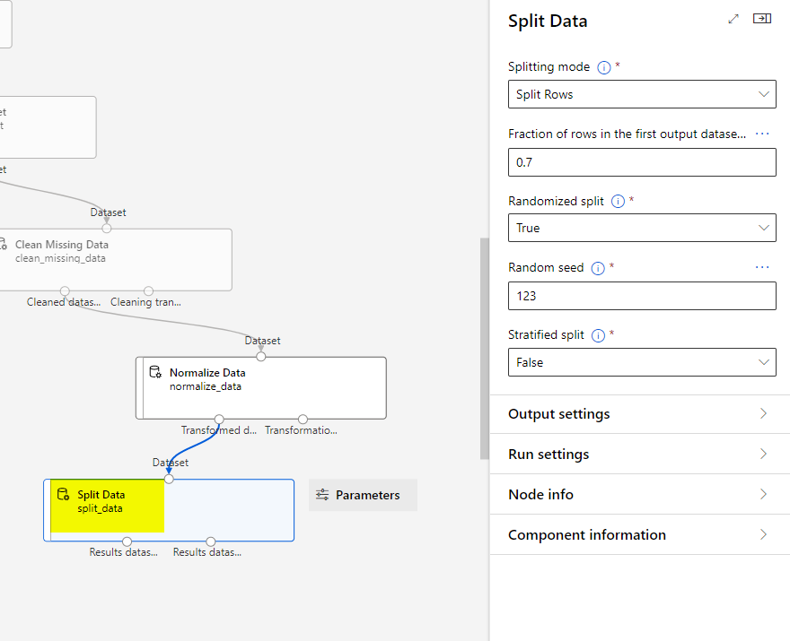
Go back to the Designer and look for a module called Split Data.
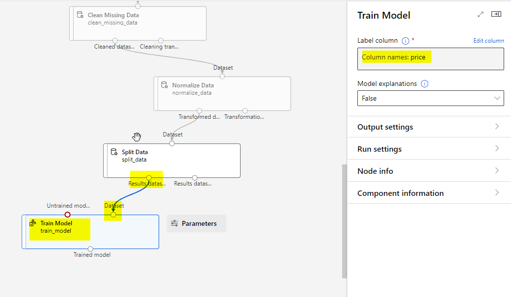
Add another module called Train Model and configure it like below:
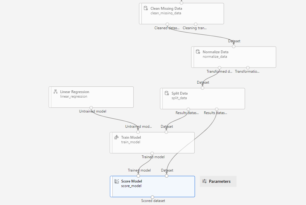
Add another Score module to test the trained module. The final diagram should look like below:
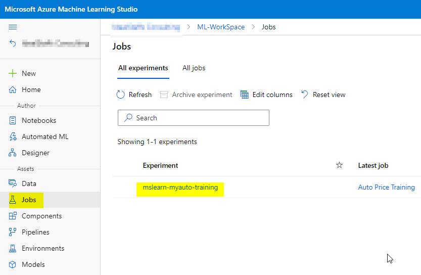
Select Submit, and run the pipeline using the existing experiment named mslearn-myauto-training.

To evaluate a regression model, you could simply compare the predicted labels to the actual labels in the validation dataset held back during training, but this is an imprecise process and doesn’t provide a simple metric that you can use to compare the performance of multiple models.
For this we need to ad an Evaluate Model module.
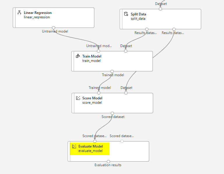
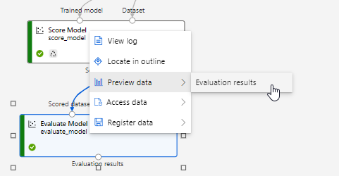
Submit again and at the end review the results of the regression performance metrics.
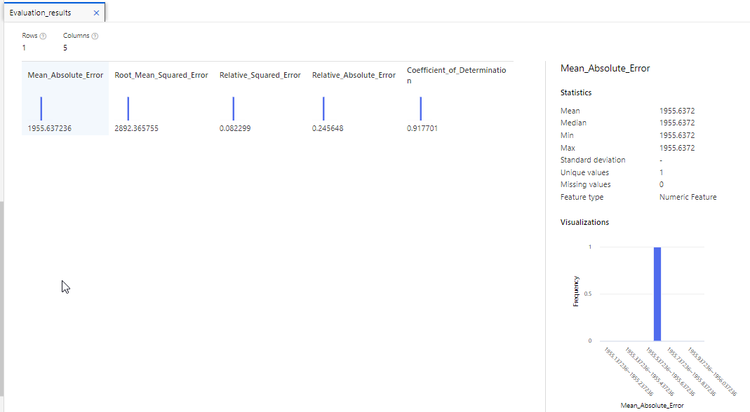
These include the following:
Mean Absolute Error (MAE): The average difference between predicted values and true values. The lower this value is, the better the model is predicting.
Root Mean Squared Error (RMSE): The square root of the mean squared difference between predicted and true values. When compared to the MAE (above), a larger difference indicates greater variance in the individual errors (for example, with some errors being very small, while others are large).
Relative Squared Error (RSE): A relative metric between 0 and 1 based on the square of the differences between predicted and true values. The closer to 0 this metric is, the better the model is performing.
Relative Absolute Error (RAE): A relative metric between 0 and 1 based on the absolute differences between predicted and true values. The closer to 0 this metric is, the better the model is performing.
Coefficient of Determination (R2): This metric is more commonly referred to as R-Squared, and summarizes how much of the variance between predicted and true values is explained by the model. The closer to 1 this value is, the better the model is performing.
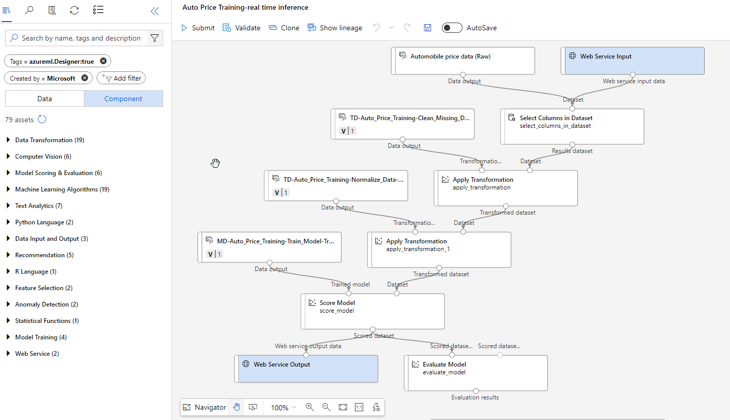
Now we need a second pipeline known as an inference pipeline. The inference pipeline performs the same data transformations as the first pipeline for new data. Then it uses the trained model to infer, or predict, label values based on its features.

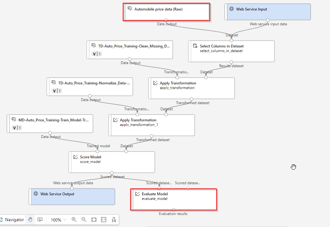
Remove the models highlighted below:
Add the following module to the design.
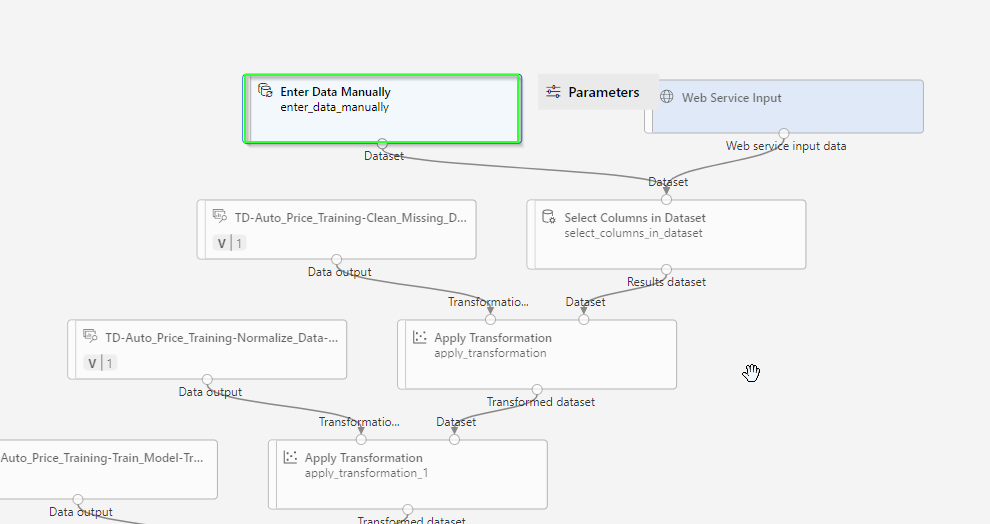
Edit the module.
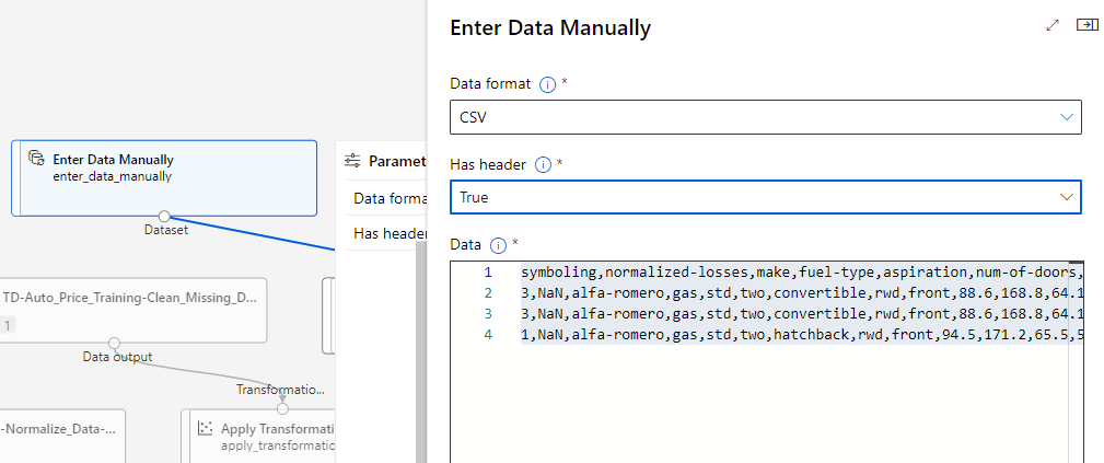
Paste the below CSV:
symboling,normalized-losses,make,fuel-type,aspiration,num-of-doors,body-style,drive-wheels,engine-location,wheel-base,length,width,height,curb-weight,engine-type,num-of-cylinders,engine-size,fuel-system,bore,stroke,compression-ratio,horsepower,peak-rpm,city-mpg,highway-mpg
3,NaN,alfa-romero,gas,std,two,convertible,rwd,front,88.6,168.8,64.1,48.8,2548,dohc,four,130,mpfi,3.47,2.68,9,111,5000,21,27
3,NaN,alfa-romero,gas,std,two,convertible,rwd,front,88.6,168.8,64.1,48.8,2548,dohc,four,130,mpfi,3.47,2.68,9,111,5000,21,27
1,NaN,alfa-romero,gas,std,two,hatchback,rwd,front,94.5,171.2,65.5,52.4,2823,ohcv,six,152,mpfi,2.68,3.47,9,154,5000,19,26
Open the module Select Columns in Dataset and remove the price column since the new data doesn’t include it and therefore we want to predict it.
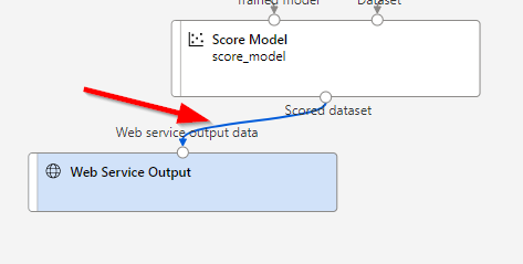
Delete the connection between these two modules.
Add an Execute Python Script module from the Python Language section, replacing all of the default python script with the following code (which selects only the Scored Labels column and renames it to predicted_price):
import pandas as pd

def azureml_main(dataframe1 = None, dataframe2 = None):

    scored_results = dataframe1[['Scored Labels']]
    scored_results.rename(columns={'Scored Labels':'predicted_price'},
                        inplace=True)
    return scored_results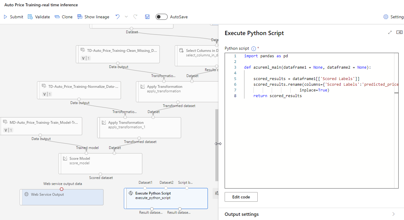
Configure the connections as depicted below:
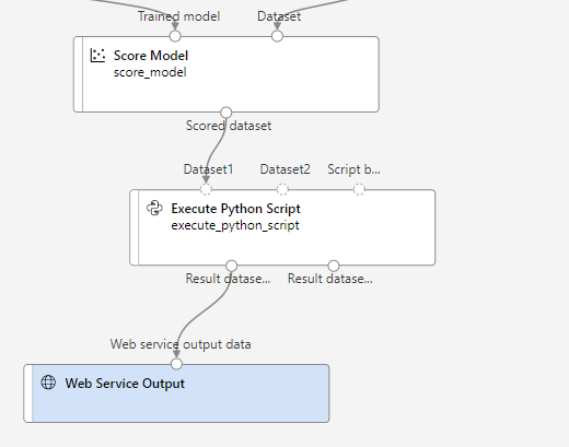
Submit the pipeline as a new experiment. When the pipeline has completed, select Job details. In the new window, right click on the Execute Python Script module. Select Preview data and then Result dataset to see the predicted prices for the three cars in the input data.
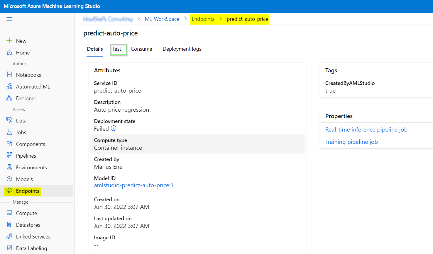
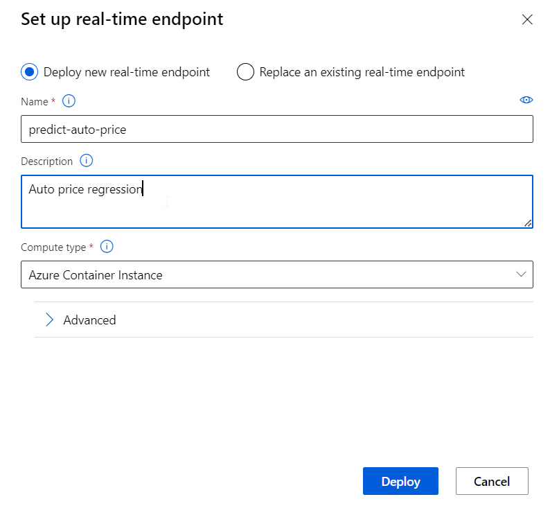
After you’ve created and tested an inference pipeline for real-time inferencing, you can publish it as a service for client applications to use.
Just click Deploy using Deploy a new real-time endpoint.
After the deployment you can click Test in order to validate and review the output.